This project attempts to predict an opponent’s strategy in StarCraft using real, in-game observations through a Bayesian network model (I think that is a fair label, but let me know if you disagree!). The actual network is represented as a tree data structure where each node represents a step in players’ build orders (more on this later). Nodes are evaluated (the probability of a certain step being taken in the game is adjusted) based on in-game observations.

Games, especially complicated games such as StarCraft where prior game states have a large impact on current and future game states (the choices I make at the start of the game decide what I can do later in the game), are often tackled using deep learning techniques such as RNN or LSTM neural networks. I believe the model described below is powerful because it is able to make predictions about highly complicated games such as StarCraft in a manner similar to neural networks while preserving a high degree of interpretability expected of Bayesian models.

I’ve divided up this discussion of the model into a brief primer on StarCraft; a description of the actual model and its implementation found in bayes_tree.py; a walkthrough of replay dataset and how strategies were determined; and analysis of an actual prediction from the model. The primer may still be helpful to those familiar with StarCraft as it addresses core assumptions the model makes about a StarCraft game.

A Quick Overview of StarCraft

StarCraft is a real-time-strategy game where two players fight to destroy the other’s army and economic infrastructure. The actual victory condition in StarCraft is the destruction of all of the opponent’s buildings, but crippling blows can be dealt by destroying the opponent’s army and/or their ability to rebuild said army. Each player begins with one base and a handful of workers who can collect resources. From there, a player must choose when to invest resources in additional bases and workers versus building military buildings and units for attack or defense.

Player strategies, especially the opening moves of a strategy, can be described as build orders. Build orders are the order units and buildings are created in. Due to buildings and units requiring resources to make, there is a large opportunity cost in making a decision to build a unit or building. For example, a barracks costs 150 minerals while workers cost 50 minerals each. I can choose to build a barracks early, but this will delay the creation of 3 workers, each of which would mine additional minerals for the rest of the game. Due to opportunity cost and “tech-trees” mandated by game-rules (I have to build one type of building before I can build another type of building), the timing and order of builds is extremely important.

I have chosen to represent each player’s strategy in a game as a series of unit/building creation decisions which we will call nodes from now on. A sequence of these nodes, ordered from first to last executed, will be referred to as a build order. Each game has two build orders which we will analyze separately. In reality these build orders will depend heavily on one another, especially in later stages of the game where players incorporate what they see their opponent doing into their own strategy, but we will treat each build order as independent for the sake of simplicity and because our model is focused on early-game strategy where the build-order is less reactive.

These build orders are not explicitly visible to the other player. StarCraft has a fog of war, where only the map in proximity to a player’s units is revealed to that player. In order for one player to figure out what his opponent is doing, he must send units over to scout out the opponent’s base. The player will end up with a collection of observations about what his opponent has constructed by various times. The model will need to use these observations to make predictions about an opponent’s strategy just as an actual player would.

As a side note, StarCraft has three factions that players choose before starting a game: Protoss, Terran, or Zerg. These factions each have their own buildings and units. I have chosen not to look at the Zerg faction since Zerg is often played more reactively and there were significant technical challenges in extracting Zerg build orders versus the other factions. The model does not assume whether the player picks Protoss or Terran – this is easily picked up through in-game observations.

The Actual Model

I designed a custom model to approach this challenge. The model memorizes build orders from game replays and represents them as a tree data structure. Build orders will overlap from the root of the tree (since all games start out the same) and form branches as nodes in each build order begin to differ from one another. The diagram below represents a simplified tree of only 4 build orders. All 4 build orders share the first 2 nodes and begin branching from there.

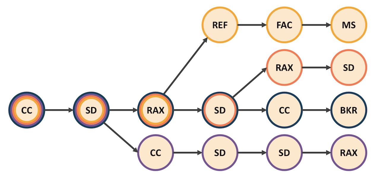
This structure is useful because it allows us to evaluate multiple build orders by looking at a smaller number of relevant nodes. The model also collects important information about each node such as the timing of the node. Each node contains the time at which every relevant build order completed that node in its respective game replay. We need to collect these timings because we will not be able to determine our opponents actual build order in-game; we’ll instead see that he has completed certain combinations of buildings and units by certain times as we scout out his base. Each node also has a frequency associated with it. The sum of child node frequencies must sum to the frequency of the parent with the ultimate root node having a frequency of 1. The idea here is that the frequency initially represents how often we saw a node get “used” in our memorized replays. For example, the root node always gets used since each game starts out the same while a node at the end of the tree likely occurred in only one replay and has an extremely small frequency.

The model is implemented as the tree class in bayes_tree.py and has three primary tasks:

• Memorize game replays to construct a tree of nodes representing all memorized build orders with corresponding frequencies and timings
• Update node frequencies based on observations in a new game we are trying to make a prediction about (discussed in detail below)
• Make a prediction. This is actually done by collecting all nodes that occur (on average) after some time and extracting a desired node attribute such as the decision each node represents or strategy (more on this later), weighted by the respective node’s frequency

The class and its methods are well commented, but I will discuss the observation updating methodology a bit. Every time we wish to update an observation, we calculate a list of relevant nodes. Relevant nodes are nodes that correspond to the decision we observe. For example, if I scout and confirm the existence of two barracks 10 minutes into the game, I will need to evaluate every node that represents the decision to build a second barracks.

The model “looks” for these nodes by starting at the root and looking down every branch, recursing as we get more and more branches. Not every branch is going to have the node we are looking for – not every strategy involves building two barracks – so we also specify a time cutoff. If the mean timing of a node is much greater than the time of my observation, I give up my search and count the node as one of my relevant nodes. Thanks to recursing at every new child node and the previously-mentioned rule that sum of all children frequencies must equal the parent, the sum of my relevant node frequencies should also be 1. This is critical because I am using these nodes to represent all possible game outcomes in the context of a particular observation.

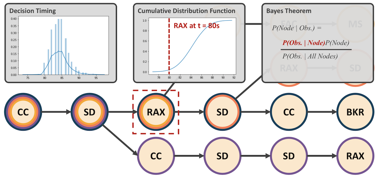
The diagram below shows how we update the frequency for a particular node using Bayes Theorem once we have all of our relevant nodes. At each node we have a collection of memorized timings which we calculate a mean and standard deviation from. This allows us to construct a cumulative distribution function which represents the probability that the node will be completed at certain times, assuming the node is completed at all. We plug our actual timing into this CDF to get P(Obs. | Node). This is divided by P(Obs. | All Nodes) which represents the sum of the prior calculation applied to all relevant nodes. This ratio is our likelihood (and the interpretable element of our model) which is then multiplied by our prior node frequency to get an updated frequency which incorporates the information from the observation.

Please note that for the nodes collected due to a timing cutoff, we assume P(Obs. | Node) = 0 as the cutoff implies that we would be approaching the left limit of whatever CDF function we might eventually construct for some children of these nodes where P(Obs. | Node) is approximately 0.

The StarCraft Dataset

I used Glen Robertson’s and Ian Watson’s dataset described here for my analysis. The researchers extracted game information on a frame-by-frame basis into a series of MySQL databases. The figure below, generated by Robertson and Watson, describes the structure of these databases.

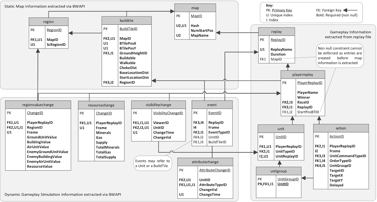
Build order information was extracted from the attributechange table as one of the attributes was whether a unit existed or not. The time of each new unit existing for the first time and the unit type were recorded to construct a full build order. The visibilitychange table was used to generate real, in-game observations for each player by recording all observations of a player by his opponent.

It should be noted that some additional logic was required to make sure the unique ID of individual units was not used to actually identify the units. In a real game, players would not be able to determine if one unit was different from another of the same type if both units were not visible at the same time. For example, if I see a marine that disappears into the fog of war, I will not know if a marine I see 30 seconds later is that same marine or a new marine unless I see two marines at once. This logic can be found in tree_predict.ipynb.

Another part of this project was trying to cluster build orders into groups of similar strategies. This was needed to evaluate the model’s predictive ability. It is not impressive to predict the next unit in a build order because often decisions are shared across very different looking build orders. For example, I am going to constantly building supply depots (think housing) for my units, whether or not I am building workers or military units. A model that tells me my opponent is likely to build supply depots is probably correct, but has not really told me much.

I’ll briefly go into the clustering here, but frankly it was just an imperfect way of evaluating the model. Clustering was done for each faction by capturing the unit composition of the player 10 minutes into every game. Each feature was the count of a certain unit type at that time. Workers were included in this unit composition to capture the general economic vs military leaning of a build order.

These unit counts were then scaled by the in-game resource cost of each unit type to make the features comparable to each other and to reflect the in-game opportunity costs of choosing to make certain units. Since clustering models are just measuring the distance between observations, we want making one big, expensive unit to have the same distance impact as making a bunch of cheaper units. This could have been approximated with standard scaling, but I think it stays true to the game to scale by resource cost.

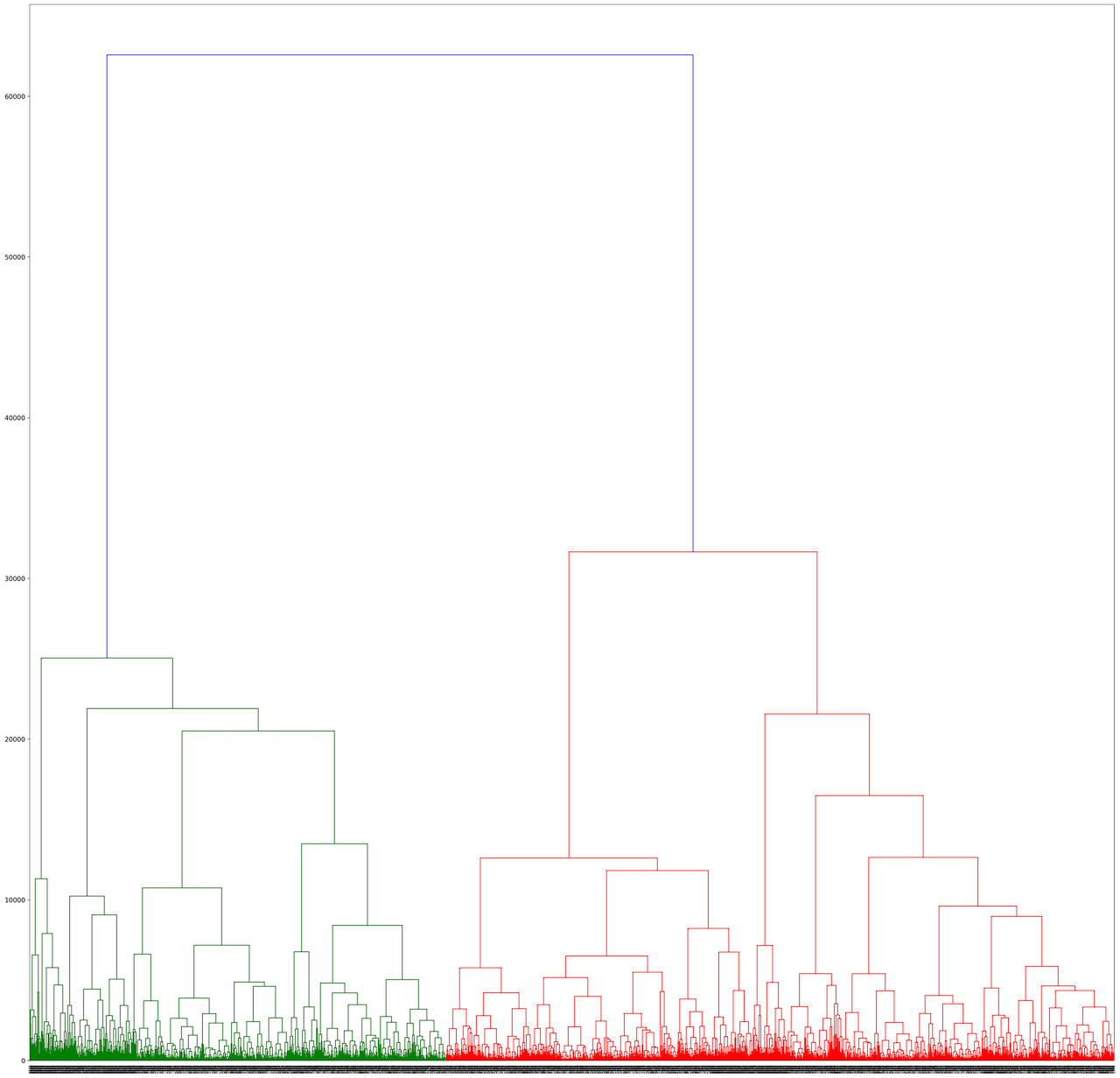
Clustering was done using a hierarchical agglomerative clustering model with ward linkages which resulted in 7 Terran strategy clusters and 6 Protoss strategy clusters. I used a dendrogram to help determine distance cutoffs. The Terran dendrogram is included as reference below.

Making Predictions for a New Game

The diagram below ticks through several observations for an unmemorized game. Please note that there were over 50 observations and these are just a few of the more relevant observations. The panels in the animation are described below:

• The top left panel shows the latest observation the model has been updated for highlighted.
• The bottom left panel shows the predicted strategy per the strategy clusters mentioned above. Each memorized build order is assigned a strategy cluster and the nodes of the memorized tree retain all strategy clusters that node is a part of.
• The right panel shows a simplified version of the tree where nodes are colored by the dominant strategy cluster of each node and opacity is determined by the node frequency.

You’ll see that nodes closer to the center are opaquer and are all one strategy as this is the main strategy seen in replays. Nodes close to the center are all more likely because a smaller number of choices must be made to reach them relative to those on the outer edge.

The start of the animation shows the full memorized tree where frequencies reflect historical replays rather than any view of the current game. As the first observation is incorporated into the model, half of the nodes are set to a frequency of 0. This is due to the tree being trained for both the Protoss and Terran factions. The observation confirms that we are dealing with a Terran rather than a Protoss player.

Subsequent observations narrow down likely build orders and therefore likely strategies that the player is following. Seeing factories implies a commitment to mechanical units while anti-air units like the Goliath signals an emphasis on air control. Sighting Vultures, units that lack an air attack, then reduces the likelihood of the strategy being air-related. By incorporating a list of in-game observations the model predicts that the mixed air control strategy is most likely, a strategy which only occurred in 3% of the historical replays.